|
The modeling process starts with sketching a model, then writing equations and specify numerical quantities. Next, the model is simulated with simulation output automatically saved as a dataset. Finally, the simulation data can be examined with Analysis Tools to discover the dynamic behavior of variables in the model.
The behavior of a simulation model in Vensim is solely determined by the equations that govern the relationships between different variables. The structural diagram od the model is a picture of the relationships between variables. Vensim enforces consistency of the diagram and the model equations.
Growth Models
We will introduce the state of the system with one stock in which rate of growth is directly proportional to the size of population.
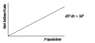
Exponential growth model
Consider the growth of the population in which the net inflow rate is directly proportional to the size of population.
Structure
 Stock and Flow Diagram
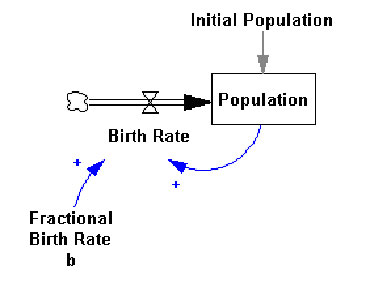 Vensim Model
- In Vensim click the New model button
- Set the Time Bounds dialog to: INITIAL TIME = 0, FINAL TIME = 10, TIME STEP=1, and Units for time=Year.
- Sketch the model shown above.
- Save your model. Name it exp.mdl
- Enter the following equations:
Birth Rate= Population*Fractional Birth Rate b
Units: people/Year
Fractional Birth Rate = 0.25
Units: 1/Year
Population = INTEG (Birth Rate, Initial Population))
Units: people
Initial Population = 100
Units: people
- Check for Model Syntax and Units Errors
- select Model | Check Model from the menu
- select Model | Units Check from the menu
- Simulate the model
- Double click on the Runname editing box on the Toolbar and tape b1 for the first run name.
- Click on the Simulate button
The model will simulate, showing a work-in-progress window until completion
Model Analysis
- Double click on the Stock Population in the sketch
- Click on the Graph tool a graph of population is generated
A key feature of Vensim is the ability to do multiple simulations on a model under different conditions to test the impact that changes in constants (or lookups) have on model behavior. Vensim also stores all the data for all variables for each simulation run, so that you can easily access information about the behavior of any variable in any run. Experiments are performed by temporarily changing constant or Lookup values and then simulating the model.
- Set up Simulation experiment of the model changing the value of the constant Fractional Birth Rate b
- Click on the Set Up a simulation button
The simulation toolbar has features specific to model simulation, allowing changes to the integration technique and buttons to change model constants and lookups.
- Click on the Runname editing box and replace b1 with the name b2.
- Click on the variable Fractional Birth Rate b (appearing blue/yellow in the sketch) and in the editing box type 0.5. Press Enter key
- Click on the Simulate button
- Click on the Control Panel button. Click the Datasets tab to open the Datasets Control and check that both runs are loaded in the right hand column. Click on the Graph tool.
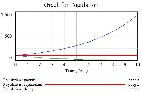
Behavior
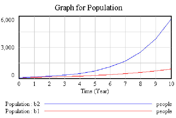
Initial population P(0)=100; Fractional Birth Rate: b1= 0.25, b2=0.5
The state of the system grows exponentially from its initial value at a constant fractional rate per time unit.
Exponential decay
Consider the change of the system in which the net outflow rate is directly proportional to the size of population.
Structure
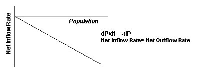
Stock and Flow Diagram
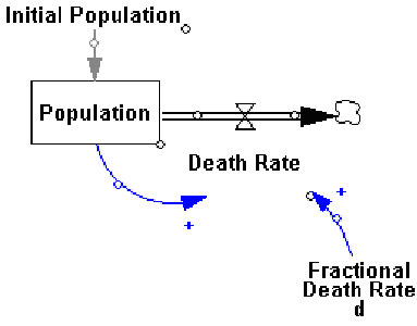
Death Rate = - Fractional Death Rate d * Population
Exercise 1. Build in Vensim a model decay.mdl, as shown in the figure above. Write equations and specify numerical quantities. What will the behavior of the system be? Create some graphs for population in Vensim experimenting with different values of Fractional Death Rate and Initial population. Explain the observed behavior
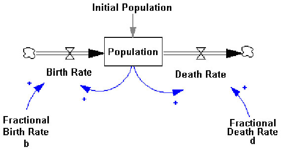
Exercise 2. Modify the model exp.mdl or decay.mdl, as shown in the figure below. Correct equations and numerical quantities. Create the graph of behavior of the system experimenting with different values of Fractional Birth Rate, Fractional Death Rate and Initial population. Explain the observed behavior.
Stock and Flow Diagram
Behavior
Analysis of the phase plots for first order linear systems shows that in systems with more than one feedback loop, the dynamics depends on which loop is dominant.
A linear first order systems can generate only exponential growth, equilibrium or exponential decay.
Logistic Growth Model
Structure
In real systems, the fractional birth and death rates can not be constant but must change as the population approaches its carrying capacity. The net fractional growth rate of the population P must fall from its initial value, pass through zero when the population equals its carrying capacity, and become negative when the population is greater than its carrying capacity. Consequently, the net births are zero when the population is zero, rise with increasing population up to a maximum, fall to zero at the carrying capacity and continue to drop, becoming increasingly negative.
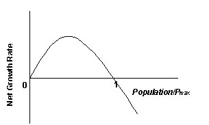
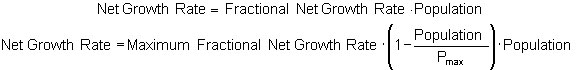
The logistic growth model posits that the net fractional population growth rate is a downward sloping linear function of the population. Let Pmax be the fixed maximum size of population that a one-species system can support. The equation for the net growth rate becomes
Stock and Flow Diagram
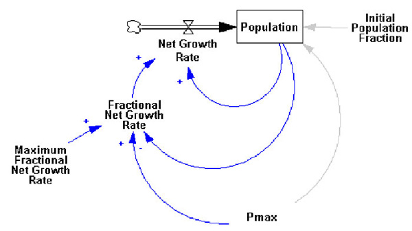
Vensim Model
- In Vensim click the New model button
- Set the Time Bounds dialog to: INITIAL TIME = 0, FINAL TIME = 15, TIME STEP=0.125, and Units for time=Period.
- Sketch the model shown above.
- Save your model. Name it logistic.mdl
- Enter the following equations:
- Fractional Net Growth Rate = Maximum Fractional Net Growth Rate * (1 - Population/Pmax)
Units: 1/Period
(The fractional net birth rate is a linearly declining function of the population relative to carrying capacity)
- Initial Population Fraction = 0.001
Units: Dimensionless
(The initial population as a fraction of the carrying capacity)
- Maximum Fractional Net Growth Rate = 1
Units: 1/Period
- Net Growth Rate = Fractional Net Growth Rate * Population
Units: People/Period
(The net birth rate is the product of the fractional net birth rate and population)
- Pmax = 1
Units: People
(The carrying capacity of the environment)
- Population= INTEG (Net Growth Rate, Initial Population Fraction * Pmax)
Units: People
(The population accumulates the net birth rate. Initialized to a fraction of the carrying capacity)
- Create the graph of behavior for population experimenting with different values of Maximum Fractional Net Growth Rate. Explain the observed behavior.
Behavior
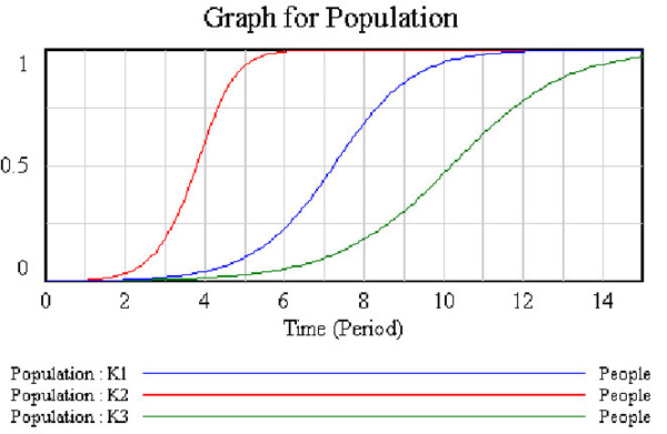
Maximum Fractional Net Growth Rate K1=1, K2=2, K3=0.7
A nonlinear first order systems generate S-Shaped growth.
The dominant feedback loops shifts as the system evolves. As the population approaches its carrying capacity the positive loops driving growth weaken and the negative loops restraining growth strengthen, until the system is dominated by negative feedback, and the population then smoothly approaches a stable equilibrium at the carrying capacity.
The structure underlying S-shaped growth applies to a wide range of growth processes, not only population growth. These include the adoption and diffusion of new ideas, the growth of demand for new products, the spread of diseases.
Modeling Diffusion of Innovations
Open the model innovation.mdl shown below.
Stock and Flow Diagram
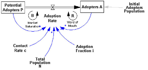
Potential adopters P come into contact with adopters at a rate of c thorough social interactions. The total rate at which contacts are generated by the potential adopter pool is then cP. The proportion of adopters in the total population, A/N, gives the probability that any of these contacts is with an adopter who can provide word of mouth about the innovation. Finally, the adoption fraction, i, is the probability that a person will adopt the innovation after exposure to an adopter.
The equations for the innovation diffusion model become:
A = INTEG(Adoption Rate, Initial Adopters Population)
P =INTEG( - Adoption Rate, N-Initial Adopters Population)
Adoption Rate = c*P*i*A/N
N = P + A
Investigate the behavior of model.
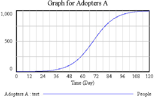
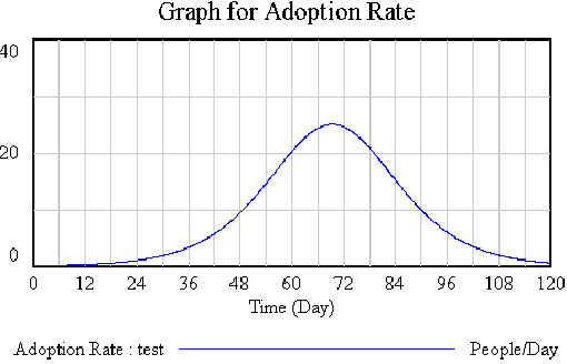
The behavior of the model is the classic S-Shaped growth of the logistic curve.
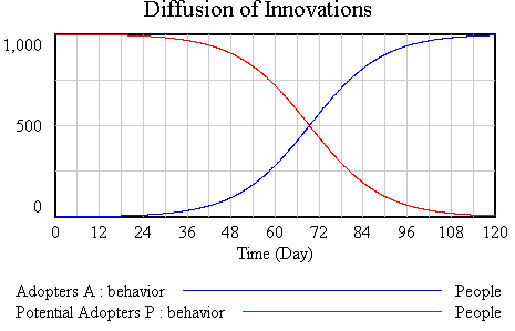
Compare the populations of Adopters and Potential Adopters creating a Custom Graph to show both variables on one graph.
Predator-Prey Populations
This models features ecology of predator (foxes) and prey population (rabbits).
This model generates interesting and insightful dynamic behavior.
Open the model RABFOX.mdl shown below.
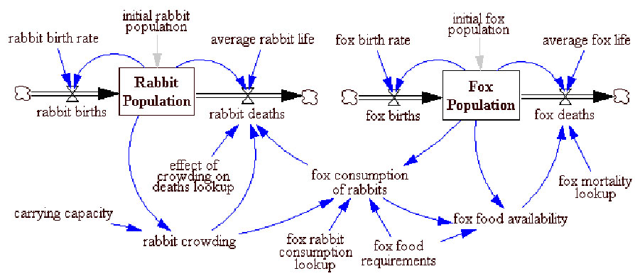
- Check equations and numerical quantities.:
- Click on the Set Up a Simulation button and choose the integration technique Runge Kutta 4 Auto. This model will not simulate properly with Euler integration. Type in a run name and click the Simulate button.
- Investigate the behavior of the Rabbit and Fox populations. Compare them separately, or create a Custom Graph to show both variables on one graph.
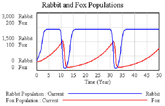
- Experiment by running simulations with values for initial fox population of 35 and 40 foxes.
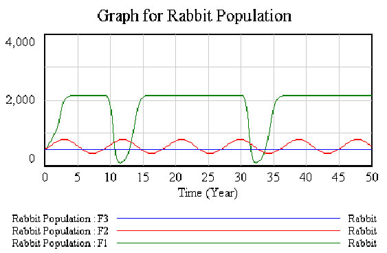
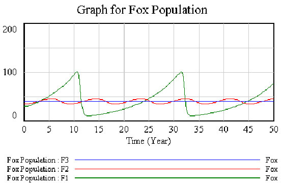
- § Compare the three different simulation runs. Explain the observed behavior.
|