Introduction

Lindenmayer-systems or L-systems are called after the theoretical biologist Aristid Lindenmayer (1925 - 1989), who studied mathematical models of plant development. The emphasis of the study initially was on plant topology, i.e. the neighbourhood relations between cells or larger plant modules. The geometry of the plant was then beyond the scope of the theory. Later, the models were extended by giving geometric interpretations to L-systems, and that turned them into a versatile tool for plant modelling. Together with Przemyslaw Prusinkiewicz, Lindenmayer also worked on the visualization of the concepts from L-systems (see references).

The central idea of L-systems is that of rewriting. By applying a set of rewriting rules or productions to some initial object, a complex object can be defined. A well-known example of such an object is the snowflake. Starting with an equilateral triangle and applying the rewriting rule that every line piece is replaced by the following figure (called the generator)

the form of a snowflake will soon appear

This so-called Koch snowflake is discussed in more detail in the chapter II.2.

The concept of rewriting rules is of course not limited to the modelling of plants. Already in the late 1950s the work of Noam Chomsky on formal grammars gave a great impulse to the study of rewriting systems, in this case rewriting systems operate on character strings. Chomsky applied the concept of rewriting  to describe the syntactic features of natural languages. He introduced four classes of grammars: regular, context-free, context-sensitive and recursively enumerable. Each grammar consists of terminal symbols (which are written  exactly as they are to be represented), non-terminal  symbols (which are defined by set of productions), and the axiom (start object).
For example:
T={a,b} /*set of terminals*/
NT={A,B,C} /*set of non-terminals */
P={p1: A→abBC
      p2: B→b,
      p3 :C→a} /*set of productions*/
applying productions to the axiom AB we get:
AB
abBCB(p1)
abbCB (p2)
abbaB  (p3)
abbab   (p4)

The four classes are summarized in the table below:


A few years later Backus and Naur provided a new notation based on rewriting rules for a formal definition of the programming language ALGOL-60 (the Backus-Naur Form or BNF). The BNF notation consists of terminal symbols, non-terminal symbols, which are defined by a BNF rules, and meta-symbols used to form those rules.
The meta-symbols of BNF are:
    ::= meaning "is defined as"
    | meaning "or"
    < >  angle brackets used to surround category names.
The angle brackets distinguish syntax rules names (also called non-terminal symbols) from terminal symbols, which are written  exactly as they are to be represented. A BNF rule defining a nonterminal  has the form:
nonterminal ::= sequence_of_alternatives consisting of strings of
terminals or nonterminals separated by the meta-symbol |
For example, the BNF production for a mini-language is:
<program> ::=  program
                   <declaration_sequence>
               begin
                   <statements_sequence>
               end ;

DOL-systems

The simplest  L-systems  are deterministic and context-free systems, the so-called  DOL-systems.  Context-free means that the productions are applicable regardless of the context in which the predecessor appears.  Opposed to Chomsky grammars, in a DOL-system  all elements in a word that can be replaced through a production rule are rewritten  simultaneously. To illustrate  this, consider the following  example. Take the set , the set of production rules and the axiom (start object) . Thus in every step is replaced by and is replaced by . This system then generates the following  gs

b

a

ab

aba

abaab

Formal Description

Let denote an alphabet. Then denotes the set of all words over and denotes the set of all non-empty words over .
A string OL-system is defined as an ordered triplet where is the alphabet, is a non-empty word called the axiom, and is a finite set of productions. A production is written as , that is the letter is replaced by the word . is called the predecessor and is called the successor of the production. It is assumed that for any letter there is at least one word such that a → χ. If for a given predecessor no production is explicitly given, it is assumed that the identity production belongs to the set of productions .

An OL-system is deterministic (DOL-system) if and only if for each there is exactly one such that .

ADVANCED
II.1a Give a formal description for the L-system  of the Koch snowflake described above.

Turtle interpretation of strings

For interpreting  an L-system  graphically several more or less sophisticated approaches exist. Here, one of these approaches is discussed: turtle interpretation. A state of the turtle is defined as a triplet , where the Cartesian coordinates specify the position of the turtle, and specifies the angle, called the heading  (the direction in which the turtle is facing). When a step size and an angle increment are given, the turtle can respond to commands represented by the following symbols

F    Move forward a step of length . The state of the turtle changes to . A line segment between points and is drawn.
f    Move forward a step of length without drawing a line.
+    Turn left by an angle . The next state of the turtle is . The positive orientation of angles is counterclockwise.
-    Turn right by an angle . The next state of the turtle is .

As an example the quadratic Koch island is taken. The quadratic Koch island can be described by the following system

In the figures below the axiom is shown in the upper left figure followed by the results of applying the production rule once, twice and three times respectively.

REQUIRED
II.1b To produce the quadratic Koch island shown above, we need to scale in every iteration the length of . What is the scaling factor?

REQUIRED
II.1c If the number of iterations goes to infinity will the area of quadratic Koch islands eventually fill the complete 2-dimensional space? Why or why not? What would happen to the length of the boundary?

Bracketed OL-Systems

In the system above the turtle interprets a character string as a sequence of line segments. The important point to notice is that the result is a single line that may or may not be self-intersecting  and can be more or less convoluted. For many structures this is not sufficient. In the plant world many structures exist with branches that cannot be described by a single line. To relinquish this limitation the turtle interpretation of strings can be extended with brackets. Two new symbols are introduced to delimit a branch:

[    Pushes the current state of the turtle  onto a pushdown stack. The information saved contains the turtle's position and orientation, and possibly other attributes such as the color and width of the lines being drawn.
]    Pop a state from the stack and make it the current state of the turtle.  No line is drawn, although in general the position of the turtle changes.

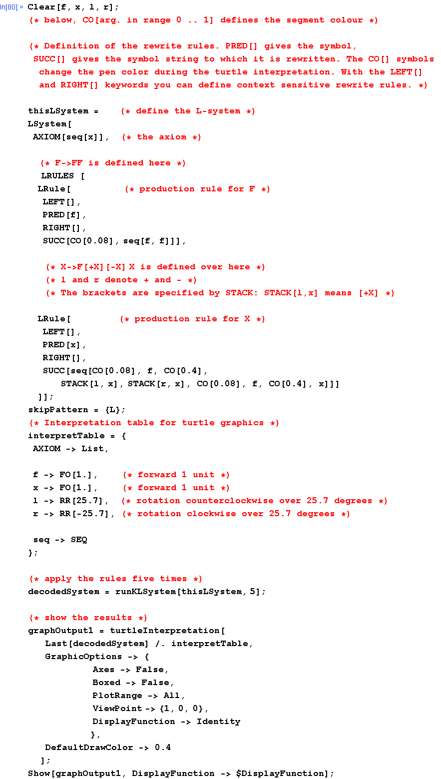
For example, the bracketed OL-system

can be used to generate the following  plant (with an angle of degrees for the rotations  and by applying the rules five times)

In this figure the F-segments are displayed in brown and the X-segments in green

The code to generate the plant (plant code) is given below

REQUIRED
II.1d L-systems have been used to model real plant growth. Modify the plant code such that a growth pattern results of a plant nearby the North Sea, with the influence of a sustained wind direction clearly visible. See for example the next figure. First explain how the rules should be adapted and then indicate the way to change the code.

Stochastic OL-Systems

Stochastic OL-systems are similar to the regular OL-systems described above, with the addition of "randomized" rewrites of rules based upon production probabilities. In stochastic OL-system productions, each predecessor may have more than one successor, with each successor having a probability associated with it. For any predecessor , the sum of all the probabilities of all productions of must be equal to 1.
For example, the following set of stochastic productions is legal input for the L-system
    Axiom:      
     Rules:      

F
F
F

In the above example note that the probabilities associated with the stochastic productions are presented above the production  arrows.

Context Sensitive L-Systems

Productions in OL-systems are context-free; i.e. applicable regardless of the context in which the predecessor appears. However, production application may also depend on the predecessor's context. This effect is useful in simulating interactions between plant parts, due to example to the flow of nutrients or hormone.
L-systems   use productions of the form -> χ where letter (called the strict predecessor) can produce word  χ if and only if    is preceded by letter and followed by and are called left and right context in this production. Production in 1L-systems  have one sided context only; consequently, they are either of the form < -> χ or    -> χ . OL-systems, 1L-systems and 2L-systems belong to a wider class of IL-systems also called (k,l)-systems. In (k,l)-system the left context is a word of length k and the right context is a word of length l.
For example, the following 1L-system makes use of context to simulate signal propagation throughout a string of symbols:
ω: öłö˛ö˛ö˛ö˛ö˛ö˛ö˛ö˛ö˛ö˛ö˛ö˛
P={ öł<ö˛ -> öł, öł->ö˛}
The first few words generated by this L-system are given below:
öłö˛ö˛ö˛ö˛ö˛ö˛ö˛ö˛ö˛ö˛ö˛
ö˛öłö˛ö˛ö˛ö˛ö˛ö˛ö˛ö˛ö˛ö˛
ö˛ö˛öłö˛ö˛ö˛ö˛ö˛ö˛ö˛ö˛ö˛
ö˛ö˛ö˛öłö˛ö˛ö˛ö˛ö˛ö˛ö˛ö˛
ö˛ö˛ö˛ö˛öłö˛ö˛ö˛ö˛ö˛ö˛ö˛
....
The introduction of context to bracketed L-systems is more difficult than in L-systems without brackets, because the context matching procedure may need to skip over symbols representing branches or branch portions. For example in the following figure it is indicated that production with the predecessor BC<S>G[H]M can be applied to symbol S in the string

ABC[DE][SG[HI[JK]L]MNO].

Although it is not visible at the first glance, ABC is the left context for S,because D, E are parts of another branch (as can be seen in the figure below). For  the similar reason G[H]M is the right context for S.This involves skipping symbols[DE] in the search for the left context, and I[JK]L in the search for right context.

Acropetal Signal Propagation

The left context can be used to simulate control signals that propagate acropetally, i.e., from the root or basal leaves towards the apices of the modeled plant. The following 1L-system simulates propagation of an acropetally signal in a branching structure that does not grow:
ignore : + -
ω : ]
< }
The propagation can be seen in the picture below:

REQUIRED
II.1e  Propose  L-system that simulates the propagation of a basipetally  signal (i.e. from apices towards the root).

Parametric L-systems

Although L-systems with turtle interpretation make it possible to generate a variety of interesting objects, their modeling power is limited by reduction of all lines to integer multiples of a unit segment.  To avoid this problem,  parametric systems were introduced.
Parametric L-systems operate on parametric words, which are strings of modules consisting of letters with associated parameters. The letters belong to alphabet V, and the parameters belong to the set of real numbers R. A module with letter A∈V and parameters , , ∈R is denoted by A(, , ). Every module belongs to the set , where is a set of all finite sequences  of parameters.
The real-valued actual parameters appearing in the words correspond with formal parameters used in the specification of L-system productions. A formal parameters can form logical (denoted by ) and arithmetic (denoted by using arithmetic (+,-,*,/), exponential (^) , relational (<>=), logical (!,&,|-not,and,or) operators and parentheses.
A parametric OL-system is defined as an ordered quadruplet G=(V,Σ,ωP) where:
V is alphabet of the system
Σ is the set of formal parameters,
is a nonempty parametric word called the axiom
is a finite set of productions
The symbols : and -> are used to separate the three components of a production: the predecessor, the condition and the successor. For example a production with predecessor A(t), condition t>5 and successor B(t+1)CD(t^0.5,t-2) is written by:
A(t):t>5->B(t+1)CD(t^0.5,t-2)
A production matches a module in the parametric word if:
1.    The letter in the module and the letter in the production predecessor are the same.
2.    The number of the actual parameters in the module is equal to the number of formal parameters in the production  predecessor.
3.    The condition evaluates to true if the actual parameter values are substituted for the formal parameters in the production.

REQUIRED
II.1f  Check if the production above matches the module A(9). Why? Why not? If yes, what would  be the result of the application  ?

Turtle interpretation of parametric words

For interpreting parametric L-system graphically we use the turtle interpretation approach as we have done for non-parametric L-systems. If one or more parameters are associated with a symbol interpreted by a turtle, the value of the first parameter controls the turtle state. If the symbol is not followed by any parameter, default values specified outside the L-system are used as in the non-parametric case.
Here is the basic set of symbols:
F(a) Move forwards a step of length a>0
f(a)  Move forwards a step of length a without drawing a line.
+(a) Rotate by an angle of a degrees

Phyllotaxis

Fibonacci series

The Fibonacci series is constructed as follows:
F(1)=1
F(2)=2
F(n+2)=F(n+1)+F(n)

Golden section

Euclid, the Greek mathematician who lived from about 365BC to 300BC wrote the Elements, which is a collection of 13 books on Geometry (written in Greek originally). It was the most important mathematical work until this century, when Geometry began to take a lower place on school syllabuses, but it has had a major influence on mathematics.
In the Elements Euclid shows how to divide a line in mean and extreme ratio which we would call "finding the golden section G point on the line".
Euclid used this phrase indicating that the ratio of the smaller part of this line (GB in the picture below) to the larger part (AG) is the SAME as the ratio of the larger part (AG) to the whole line AB: =

If we let the line AB have a unit length and AG have length g (so that GB is then just 1ńg) then the definition= means that :
, or =1-g
The solutios of this equation is
g= or

For our geometrical problem, g is a positive number, so the first value is the one we want.

REQUIRED
II.1g  Let AG have a unit length and GB length x, so that AB now has length 1+x. If Euclid's "division of AB into mean and extreme ratio" still applies to point G, what quadratic equation do you now get for x? What is the value of x? How does it compare to g?
REQUIRED
II.1h The value of x obtained in the previous exercise is called golden section and is usually marked as . Show that
lim

ADVANCED
II.1i  Repeat the calculation to find  the golden angle  (the ratio of the value of the golden angle ϕ to the angle 36-ϕ is the SAME as the ratio of the 36- ϕ,  to the full angle 36 ). Prove that .

Phyllotaxis - a simple model

The elements of plant (leaves, sepals, florets, etc) form very regular lattices, with crystalline-like order. In the most common arrangements (e.g., on a sunflower head or a pinecone), one can see conspicuous spirals linking each elements to its nearest megabars. The whole surface is covered with a number i of parallel spirals running in one direction, and j in the other. The most striking future is that (i,j) are nearly always two consecutive numbers of the Fibonacci series.

One of the first models explaining such patterns was a Vogel's model (see H.Vogel. A better way to construct the sunflower head. Mathematical biosciences, 44:179-189,1979) that proposes a relation:
,
where:
n is the ordering number of a floret, counting outward from the center. This is the reverse of floret age in a real plant.
φ is the angle between a reference direction and the position vector of the floret in a polar coordinate system originating in the centre of capitulum. It follows that the divergence angle between the position vectors of two successive florets is constant,
r is the distance between the center of the capitulum and the center of the floret, given a constant scaling parameter c .
The square root relationship between the distance r and the floret ordering number has a simple geometric explanation.  Assuming that all florets  have the same size and are densely packed, the total number of florets that fit inside the disk of radius r is proportional to the disk area. Thus, the ordering number n of the most outwardly positioned floret in the capitulum is proportional to or . The divergence angle of is much more difficult to explain. In the simple model presented by Vogel this result was derived using two assumptions:
a) Each new floret is issued at a fixed angle α with respect to the preceding floret.
b) The position vector of each new floret fits into the largest existing gap between the position vectors of the older florets.
The parametric L-system built according to the Vogel's formula ('*' means "matches every condition"):
#define a 137.5 /*divergence angle*/
#include D /*disk shape specification*/
ω=A(0)
P={A(0):⋆ ->+(a)[f(n^0.5)~D]A(n+1)}
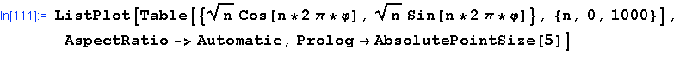
Below, the Mathematica code to generate a sunflower's head using Vogel's formula is presented:

REQUIRED
II.1j Using the Mathematica code above:
a) Try to find out the shape of the sunflower  if ϕ= 0.5 and 0.6
b) Are these seeds still  densely packed? Why?

Phyllotaxis - an advanced model
The more advanced model was introduced by Douady and Couder (see S.Douady and Y.Couder, Phyllotaxis as a Physical Self-Organized Growth Process. Phys. Rev. Lett. 68(13) 1992) who investigated the process of growing of primordia (which will evolve into leaves, pentals, staments, florets, etc.) at the apex. Due to growth, the existing primordia are advected away from the apex while new ones continued to be formed. Douady and Couder made the following assumptions:
a) Identical elements are generated with periodicity T at the given radius from a center in a plane surface. They are radially advected at velocity
b) Each element is a particle  generating a repulsive energy E(d), where d is a distance to the particle. (Several energy laws were used , , ).  To decide the place of birth of a particle, in each point of the circle C the value of total energy was computed due to previous particles, and place the new element at the point of the minimum energy.
Parameter G =   describes by how many previous particles a new particle is repelled by. Douady and Couder simulate the system numerically. They fixed the value of G and began with any previous particle to see which pattern is spontaneously obtained. They also initially forced an artificial pattern for different values of G and observed whether it could keep growing. They found out that the main curve plotting ϕ(G) (where ϕ is the angle between radial direction of two consecutive elements in each pattern) goes to the golden angle, when G goes to 0 (that is a new particle is repelled by all previous particles).